Introduction to R: Control Structure in R Part 1

In our previous discussion, we talked about other textual formats in R. In this blog we will discuss about the control structures which are commonly used when writing a R program, these structure ensures the control of flow in the R Language. There are several control functions that we will discuss here:
a. if and if, else - used to test a condition.
b.  for loops-  used to execute a loop for a fixed number of times.
c. while loops - used to execute a loop "while" a condition is proven true.
d. break - used to break an execution of a loop.
e. next - used to skip an iteration of a loop.
f. return - used to exit a loop.

Control Structure 1: if () {} else{} & if (){}, else if(){} else{}

The if(){} and if(){} else{}  function tests a logical condition. If the conditions are set to be true, the program will execute a command. If the conditions are set to be false, R will execute another set of commands.

The simplest form of the if(){} control structure is in the form of:

if(Condition){command

}else{

}

For two conditions the if(){}, else if {} structure takes in the form of:

if(Condition 1){command 1

} else if(Condition 2){command 2

}else{

}

If you have observed, the else{} syntax is usually written after each command.

For multiple conditions, then it is obvious that the control structure looks like:

if(condition 1){command 1}

if(condition 2){command 2}

if(condition 3){command 3}

if(condition 4){command 4}

.

.

.

.

.

if(condition N){command N}

the else{} is not necessary in the multiple conditions.

Control Structure 2: for(){} Loops

The for(){} loops is the most common type of looping operator in R. In this operator, there is a loop index which is commonly termed as i, however for multiple loops, the index can take the form of other letters ( k,l,m,n,o,p, etc.). The for(){} loops take an iterator variable and assign into it successive values from a sequence or vectors. the for(){} loops are commonly used over the elements of an object.

The simplest for(){} loops takes the form of:

for(){

command

}

Example 1:

Create a for(){} loop that will loop over numbers 1 to 20.

In this example, the loop takes the variable i and in each iteration of the loop it will print out a value of 1 to 20. After the last number is printed out, the command exits.

Example 2:

Create a  for(){} loop that will loop using the index i, which is sequenced from 1 to 5, the loop will print out the ith element which corresponds to the letter "a", "b", "c", "d", "e".

Example 3:

The seq_along() function takes over a vector as an input and creates an integer sequence which is equal to the length of the vector. Using the previous example, Example 2., we have a vector of length 5 if the seq_along() is used the command will create a vector sequence 1 to 5.

Example 4:

Using the previous example, Example 2., we will create a different index variable and call it "alphabet". This index variable will be taking values from an assigned vector, hence, the index variable does not need to be an integer (since it can take elements from any arbitrary vector). In this example, the for(){}loop is going through the vector c with values "a", "b", "c", "d", "e" and printing out the index variable which is equal to the letter.

Nested for(){} Loops

A nested for(){} loops is similar to having a for(){} loops existing inside another  for(){} loop.

Example 5:
In this example we will create a matrix with 2 rows and 3 columns. The command will loop over the column with the outer loop that is the "i" index. This, "i" index will loop over the rows. Using the seq_len() function over this "i" index, we have created an integer sequence over the rows. Using another seq_len() function over the "j" index to take the number of columns and create an integer sequence over the column.

A word of caution, be careful when using nested for loops and never go beyond 2 to 3 levels as this will make the command difficult to understand by others.

Introduction to R: Other Textual Formats in R

Last time we discussed on how to save a .csv file. In this blog we will discuss on other textual formats that is present in R, these are basically functions that can be used for other formats aside from .csv or .txt.

There are two functions that can be used to read or write other textual formats in R, these is the dump() function and the dput() function. These two functions are important for reading and writing other textual formats because it makes these formats editable and recoverable. The downside with dump() and dput() functions is that they are not space efficient.

The dput() Function

This function is another way to pass data into R by desparsing R objects. The dput() function can be read by dget(). The mechanism of the dput() function is that it will take an R object and will create an R code that will essentially reconstruct the object in R.

Example:

We will create a small data frame with two columns. The first column will be named "d" and the second column is named "f". The value of a will be set to 10, will the value of b is set to "d".

In the first part of our example, we have the expression z<-data.frame(d=10, f="d"). If the data frame is in dput() function, it will reconstruct the R code creating a list with two elements, the new construct has the class at the end, as you can see in the example: class="data.frame". Another essential thing is that for us to retrieve this expression, we must dput it into a file, as in the example dput(z, file="z.R"). The file can now be retrieved using the dget() function, in the example it is x<-dget("z.R"). Hence, dput() function essentially writes an R code which can be used to reconstruct an R object.

Dumping Objects in R

If we have multiple objects that we want to desparse in R, we can use the dump(c(), file=" ") function. Dumping is quite similar to dgetting, the main difference is that dumping is used in multiple objects while dget is used for single objects. R passes the dump as a character vector which contains the name of the object.

Example:

We create two objects, x and y. We assign a string vector "owl" to x and a data frame (a=10, b="a") to y.

Introduction to R: Saving an Excel File as CSV

In the previous post we talked about loading and writing files in R, we also tackled the topics about the read.table() and the read.csv() functions. In this post we will learn how to save an Excel file in csv format.

CSV is short for comma separated values, this allows the data to be saved in a table structured format. Excel files that are saved under the csv format takes the form of a text file containing information separated by a series of comma between values.

The R language however can read other file formats:
read.xls() for the Excel files, though you need to have a Perl run time to exist in the system to use this. A more complex form of importing Excel files to R is through the use of the loadWorkbook(), to load the workbook and the readWorksheet() to open the desired worksheet in the workbook. You need to install Java for this.

To import Minitab files to R you can use the read.mtp(), for SPSS R Language has the read.spss() and finally for the csv we have the read.csv().

Before you can load your csv in the R language you need to save your Excel files to the csv format using the following steps:

a. In this example I have an Excel file which contains the current employee census of Australia.

b. Click the home button, click Save as, click Other formats.

c. Choose the CSV(comma delimited) format. You have an option to chosse the CSV(Macintosh) or CSV(MS-DOS). I prefer to use the comma delimited format.

d. Click Save.

e. If you have multiple sheets, Excel will give you a warning that only the current active worksheet will be saved into the csv format and other worksheets should be individually saved.

f. Another warning will pop out that the file may not be compatible with the comma delimited format, you can ignore this and click yes.

Introduction to R: Loading Files, Writing Files, and the read.table() and read.csv() Function in R

In our previous discussion we talked about the the ways on how to remove NA values in R. This time we will talk about the different ways of loading and writing files in the R Language. The following are the principal functions for loading, and writing ready-made data into R.

For  loading tabular data, such as those in the excel format:
read.table()
read.csv()

For loading lines in a text file:
readlines()

For loading a R code file:
source(), which is the inverse of a dump as we will later discuss.
dget(), which is the inverse of a dput which will be discussed later.

For loading files that are saved in the workspace:
load()

For loading single R objects in a binary code:
unserialize()

For writing tables in R:
write.table(), although a common thing we do is to write the data in the form of a data frame.

For writing lines in R:
writeLines()

For writing codes in R:
dump()
dget()

Saving R files in the workspace:
save()

For writing a binary in R:
serialize()

read.table()  & read.csv()Function in R

The read.csv() is identical to the read.table() function the only main difference is that the read.csv() has a comma as a separator while that of the read.table() has a space as a separator between each values. The read.csv() is a common format from excel files.

The read.table is suitable for small or moderately sized data and has the following common arguments:

file() is used to determine the name of file or name of connection.

header() is a simple logical command if the file contains a header line.

sep() is a command that determines how the data in the table are separated.

colClasses() is a command that indicates the class of each column in the data set.

nrows() is a command that indicates the number of rows in the data set.

comment.char() is a string of character that is indicating a comment.

skip() is a command that skips a number of lines from the previous text.

stringAsFactors() is a command that encodes a character variable as a factor.

As previously said, the read.table() function is suitable for small or medium size data, but in cases where analyzing large sets of data are needed the following precautionary measures should be done:

a. First, calculate the memory required to read and store the large data.

To make a rough calculation on the memory needed by your large data follow the formula:

Memory Requirements = number of rows x number of columns x (8 bytes per objects)

Total Memory Requirement = 2 x Memory Requirements

b. Second, remember that R's operation is dependent on the amount of RAM in your computer.

c. Third, it is better to close other applications on the computer to avoid the delay in the R operation.

d. Fourth, use colClasses to specify the classes in the columns, this will orient R the classes of objects in the column.

e. Fifth, cut your data into tidbits when analyzing:

- take the first 100 rows.

- Loop through each column using sapply() function.

- Use the taball operator to determine what classes are present in each column.

the format is as follows:

initial<-read.csv("name of file here", nrows=100)

classes<-sapply(initial, class)

tabAll<-read.csv("name of file here", colClasses=classes)

Introduction to R: Removing NA Values

We have discussed sub-setting objects and elements in our previous topic. Now we will discuss on how to remove NA or missing data in R. This is the most common operation in data analysis because most of the raw data have missing values. The principle is to create a logical vector that will locate the NA values, these NA values are then removed using the [!] operator.

Let's proceed to the exercise:

Say you have a list x<-c(1,NA,3,NA,NA,6,NA,7,8) and you want to remove the missing values. In our previous discussion on missing values, there is an is.na() function whose purpose is to locate the missing values in your vector. We will create a logical vector z<-is.na(x), this logical expression will determine the location of the NA values, to remove the NA values we will use the [!] expression in the form of x[!z].

REMOVING NA VALUES IN MULTIPLE VECTORS

If you have more than one vector with missing values, you can use the complete.cases() function. For example:

You have two vectors x<-c(2,NA,4,NA,6,NA,8,NA) and y<-c("b", NA,"d", NA,"f",NA,"h",NA). We will create a logical vector that will give an output with deleted NA values using the expression: z<-complete.cases(x,y).

REMOVING NA VALUES FROM A DATA FRAME

In most of the cases our data are stored in tabular forms such as in .xls files or in csv files. For this exercise we will use a csv file to create a data frame in R. The data from this .csv file is from a quiz used by the John Hopkins School of Public Health and Biostatistics titled "air quality", download the file here.

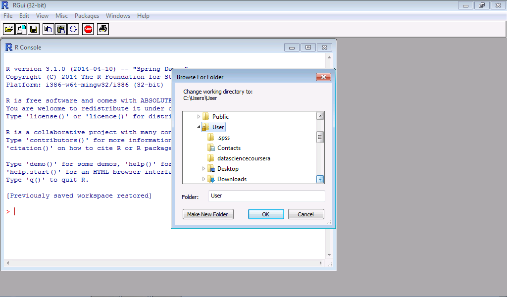
Step 1: In your R console click File.

Step 2: A menu box will open, click Local Disk (C:)

Step 3: Click the directory Users.

Step 4: Click another directory named Users.

Step 5: The file you have downloaded should be in the Download directory, click this folder then click OK.

Step 6: To determine if the file is in the Download directory type list.files(). The air quality file should be present.

Step 7: To read the data from the file type read.csv("airquality.csv"), the R console will show a data frame which consists of 153 rows and 6 columns (Ozone, Solar.R, Wind, Temp, Month, Day).

Step 8: Say we only want to analyse the first 10 rows, then we type airquality[1:10,]. Recall in our previous topic on matrices, rows have the syntax [nrow,] while the column has the syntax [,ncolumn]

Step 9: If you have observed there are NA values in the data frame, to remove the NA values we type the expression z<-complete.cases(airquality). To give an output where the NA values are removed we type airquality[z,][1:10,].

As you have observed all the rows with an NA values are deleted and are replaced with another row with complete data sets, but there are still 10 number of rows.

Introduction to R: Sub-Setting Part II

Previously we have discussed about sub-setting an object or an element in R. Now we will discuss on how to sub-set objects and elements from a list. The principle are the same the operators [], [[]] and $ can be used.

Let's proceed to the exercises. Create a list with two elements, name the first element with your first name and assign a value to it with the sequence 1 to 5. Name the second element with your favourite fruit and assign your favourite number as its value.
a. Extract the first element in list form.
b. Extract the first element in sequence form.
c. Extract the second element using $ and [[]] operators.
d. Extract the second element in list form by using the name of the element of interest.

The operator [] returns an output with the same class as the original, since x is a list then the expression x[1] will give an output that is also a list with a sequence 1 to 5. The [[ ]] operator only gives an output which is a sequence of the numbers 1 to 5.

You can also use the name of the element inside the [] operator, as in the ["durian"] example, here we use the name "durian" instead of the number index 2.

The [] operator can also be used to extract multiple elements from a list using the [c()] function. Let's proceed to the exercises:
Create a list with three elements, name the first element with your first name and assign a value into it with the sequence 1 to 5. Name the second element with your favourite fruit and assign your favourite number as its value, name the third element with your favourite animal and assign a value which is equivalent to the number of its legs.
a. Extract the elements 1 and 3 from the list that you have created.

Here we have made the expression x[c(1,3)], 1 being the number index of the first element which corresponds to the name gerard and 3 being the number index of the third element in the list which corresponds to owl.

It should be noted however that the [[ ]] and the $ operators have different function when used to retrieve an element from a list. The [[ ]] operator can only be used with a computed index while the $ operator can only be used with a literal name. Let's take the above example:

Here we have made a new vector x<-"gerard", the purpose of this is to create a vector to assign the values of the element gerard=1:5. The x<- expression resulted in a computation that the string "name" is equals to the string "gerard".  Notice that the list x only constitute the elements "gerard", "durian" and "owl" but there is no element "name", hence the x[[gerard]] becomes similar with the x[[names]].

However, if we use the x$gerard, the operation $gerard will literally look for the string "gerard" in the list, thus x$gerard is not equivalent to the x$name, if you have observed that when we type the x$name it gives out a null because the string "name" does not exist in the original list: x<-list(gerard=1:5, durian=7, owl=2).

SUB-SETTING ELEMENTS FROM A LIST NESTED INTO ANOTHER LIST

The [[c(number index, number index )]] operator can be used to extract an element from a list that is nested within another list, to illustrate this we go to our next exercise.

Say, we want to extract the number 5 from the expression:

x<-list(gerard=list(1,3,5), durian=list(2,4,6), owl=list(7,8,9)).

As you can observe the number 5 is the third element of a list named "gerard", furthermore, the list that is named "gerard" is the first element of another list which is "x". To extract the number 5 we need to use the number index method we previously discussed. The number index of the number 5 in the list "gerard" is 3, while the number index of the list "gerard" form the original list "x" is 1. 

Using operator [[ c()]], the expression becomes x[[c(1,3)]]. 1 for the number index for "gerard" and 3 for the number index of "5".

PARTIAL MATCHING IN R

If you have a list with an incredibly long name and you want to save time in typing, you may opt to use the operators: [[ ]] and $. 

For example we have a list containing the elements pneumonoultramicroscopicsilicovolcanosis having the sequence 1 to 5, the second element is another long name monosodiumglutamate with the sequence 6 to 9 Since it would take us time to type the word  pneumonoultramicroscopicsilicovolcanosis over and over again every time we want to know its value we can use the expression $p.

The $p expression will search for a name in the list containing a word with p as its first letter.

Care should be taken as R program is quite syntax sensitive, as you can observe X$p and x$P will give a NULL value. On the other hand,  the [[ ]] operator has a different approach, as you can see if you type [[ "p"]] gives out a NULL this is because the [[ ]] operator will search for an exact match in the list, since the list x do not have an element named "p", the result is a NULL, to resolve this we can use the [[ , exact=FALSE]] operator, like in our example x[[ "p", exact=FALSE]].

Introduction to R: Sub-setting Part I

In our previous discussion we talked about factors, missing values, data frames and naming. In this session we will talk about sub-setting elements in R. Sub-setting is useful if you have a manageable set of data, the operation is helpful when you want to know what element is present on a particular location in your list, vectors or matrices.

There are three operators for sub-setting objects in R:
[ ] is used to extract an object of the same class as the original, by this we mean that if you want to extract a list form a list, the output is a list, or, if you want to extract a character element from a vector the output is a character element.

[[ ]] is used to extract a single element from a list or a data frame. The class of the output is not necessarily the same as the original. It means that if you extract a numeric vector 1 from a list, the output may not necessarily be a numeric vector 1, it can be an integer 1 or a character "1".

$ is used to extract elements from a list or data from that has a name. Remember, in our previous discussion, names are useful to reference an object. Again, the class of the output is not necessarily the same as the original. It means that if you extract a numeric vector 1 from a list, the output may not necessarily be a numeric vector 1, it can be an integer 1 or a character "1".

Let's go to some exercises:
1. Express a character vector having the element a to d.
2. Extract the 1st element, 2nd, 3rd and 4th.
3. Extract all the elements other than a.

Solution:
We can actually do this in two ways, first we can use the numeric index method. In this method R recognizes each element of the character vector with a number say "a"=1, "b"=2, "c"=3 and "d"=4. If we type x[1], x is the vector of interest and [1] is the 1st element within the vector of interest, if we hit enter it gives us an output of "a".

To solve the next problem, we can use the logical index method. By default, R can recognize lexical ordering, that is c>b>a or a<b<c<d<e and so forth, by using this default we can create a logical indexing. Since b,c and d are greater than a we can let y be anything that is greater than a. The expression is y<-x>"a", in this case the expression x>"a" is coercing the values b,c,d to the vector of interest which is x, the expression y<-x gives a new variable vector which is y which will nest all the values from the vector if interest which is x, in this case all values greater than a.

The output for y is actually a series of logical values: FALSE TRUE TRUE TRUE. The first one is FALSE because "a" is not greater than "a". To determine which are greater than a the x(y) function is used and the output is a series of letters that is greater than "a".

Next, we will learn on how to sub-setting a matrix. Matrices can be sub-setted with the (row, column) type index. Let's jump to the exercises.
Ex:
a. Construct a 2 by 3 matrix with a number sequence 1 to 6. 
b. Extract the element of row 1, column 2.
c. Extract the element of row 2, column 1.

The solution is simple and the expression x[row, column] is used to extract the element of interest. Let's go further, say we want to:
d. Extract all the element of the first row only.
e. Extract all the elements of the second column only.

Remember in our previous discussion on data frames that the number before the comma represents a row and any number after the comma represents a column; so [1,] is row 1, [2,] is row 2 and so on while [,1] is column 1, [,2] is column 2 and so on. The same expression goes to extracting all the elements of a row or a column in a matrix, using the expression x[row number,] or x[, column number]. so we have x[1,] to extract all the elements at row 1 and x[,2] to extract all the elements at column 2.

By default when an element from a matrix is extracted or sub-setted, R usually gives a vector output. But what if we want the output to be a 1x1 matrix, how can we do this? The expression x[row number, column number, drop=FALSE] can be used. So let's go on to some more exercises. Let's take the previous problem, and say we want to:
a. Extract the element of row 1, column 2.
b. Extract the element of row 1, column 2 in a matrix form.

c. Extract the elements of row 1.
d. Extract the elements of row 1 in matrix form.

Introduction to R: Factors, Missing Values, Data frames and Names

In our previous discussion, we learn on how to create vectors, matrices and lists in R, now we will learn about factors, missing values, data frames and names in the R language.

We will first discuss what are factors. Factors are ways to represent categorical data in R, a categorical data can be an unordered nominal data such as gender, color or flavor, or an ordered ordinal data such as 1st, 2nd, 3rd, 4th, 5th. Factors are important in modelling functions such as lm() for linear modelling and glm() for generalized linear modelling. Factors are self-describing such as male or female for nominal factors, senior level, mid-level or junior level for ordered factors.

A factor can be created in R using the factor() function, the input of a factor() function is a character vector. Say for example, we want to create a factor with two levels: yes and no, we then want to create a frequency table on how many no's and yes's are present.

The table() function is used to determine the frequency of the yes and no's in our example. The unclass() function gives a default output that is innate in R, 1 being no and 2 being yes, the unclass() function also gives the attributes that is involved in the expression.

R usually determines the baseline function in an alphabetical manner, in the yes and no example the baseline is no. However during modelling, ordered baseline factors are quite important. To create an ordered factor in R we need to use the levels=c() function. In our previous example if you have observed in the unclass(x) attr(,"level") the output starts with a no followed by the yes, this is because in the alphabet the letter n comes before y, so the baseline factor here is no. But what if we want to have yes as our baseline factor? 

Here we integrated the levels=c("yes", "no") expression in the factor() function, the first character "yes" tells R that the baseline factor will be "yes", as can be observed in the Levels output that started with a yes, Levels: yes no.

Most of the time you will often encounter factors with a missing value. Missing values are a special kind of objects in R which are defined as NaN if it is an undefined mathematical operator or a NA if it is a missing value or an error. To test for a missing value or an error, the is.na() function can be used, while for undefined mathematical operators the is.nan() function is used.

NA values can have a class, it can be an integer NA, a character NA, a numeric NA, a logical NA, or a complex NA. A NaN value can be a NA but a NA value can never be an NaN as seen in our example. We have also seen that the output is a logical vector: true if there is a missing value or an undefined mathematical operator and false if NA or NaN is not present.

Another component in R is its ability to create or read data frames, these function is used to store and analyse tabular data. It is represented by a special type of list where every element on the list has the same length. Each element of a list is given as a column while each length of an element in the list is given by the row. Data frames can store different classes of objects in each column, unlike matrices which requires that each element should be of the same class. R can read data frames by the read.table() function or the read.csv() function. Data frames can also be converted into a matrix by the data.matrix() function.

Aside from reading tables and text or csv files, data frames can also be created in R using the data.frame()  function.

In our example we created a tabular data frame with a number sequence 1 to 3 and followed by a logical sequence of False, True, False. The first object number=1:3 is taken as the first column and the logic=c(F,T,F) is taken as the second column. The nrow() and the ncol() function can be used to determine how many rows and columns are there in the expression.

Aside from data frames, we can create readable codes and self-describing objects in R by the name() function. Say for example we want to create an integer vector from 1 to 5, we will name each integer: cat, dog, ant, bird, tree.

Lists and matrices can also be named as in the following examples:

naming list is quite direct, just by placing the names inside the list() function.

For naming matrices the dimnames() function is used using the list(c()) function as a variable. A matrix expression is first constructed specifying the number of sequence, the number of rows and columns present in the matrix. This is followed by the dimnames() function, as can be observed the first two names ("cat", "dog") are taken as row names, while the ("ant", "bird") are taken as column names.